4.5 Instrument Performance Models

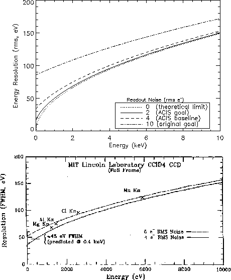
Theoretical and measured spectral resolutions are shown in Figure 4.6. Different relations are shown for a range in system noise.

**Figure 4.6:** ACIS theoretical and measured spectral resolutions
$\begin{figure} \centering\leavevmode\epsfxsize=4truein \epsfbox{ACISplots/acis... ...ring\leavevmode\epsfxsize=4truein \epsfbox{ACISplots/acismsres.eps}\end{figure}$

The theoretical energy resolution for a single event entirely absorbed in one pixel is described by

$\begin{displaymath} \Delta E = 3.65\sqrt{8\ln 2}\sqrt{N^2+FE/3.65},\end{displaymath}$

(23)

where $\Delta E$ is the FWHM of the detected peak, E is the energy, 3.65 is the energy in eV per electron released, N is the amplifier root-mean-square read noise in electrons, and F is the Fano factor.

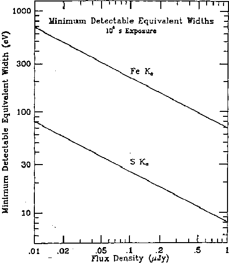
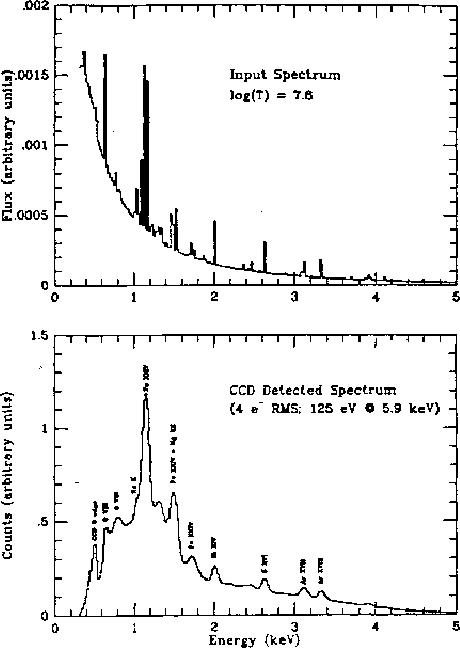
Figure 4.7 shows minimum detectable equivalent widths, and Figure 4.8 shows model spectra. Energy resolution depends critically upon the efficiency of counting only single events (see Operating Principles [Section 2.3.1.1]), but also upon CTE, bias correction accuracy, and thermal stability.

**Figure 4.7:** ACIS minimum detectable equivalent widths
$\begin{figure} \centering \leavevmode\epsfxsize=4truein \epsfbox{ACISplots/acismineqw.eps}\end{figure}$

**Figure 4.8:** ACIS model spectra
$\begin{figure} \centering\leavevmode\epsfxsize=4truein \epsfbox{ACISplots/acissimspec.eps}\end{figure}$

Because of the many factors affecting instrument performance it will be necessary to provide individual response models for at least every CCD chip and possibly every CCD output node. In practical use these models will take the form of response matrices, compatible with commonly used X-ray analysis packages such as XSPEC and PROS. Unfortunately there is no simple analytic conversion to be able to transform empirical calibration data into response matrices. Instead we utilize a simulation based on physical parameters of the CCD devices, filters, HRMA and other relevant parts of AXAF, and compare the results of the simulation to the calibration measurements.

Once acceptable agreement is found between the simulation (after physical parameters have been adjusted to reasonable levels and the simulation reaches an acceptable level of detail), the simulation is used to generate response matrices and predictions of ACIS performance on scales or parameter values which are impossible to empirically measure. In the next section we describe this simulation tool.