4.5.3 Sub-Pixel Position Reconstruction

The FWHM of the HRMA PSF was measured to be roughly 0.5 arc-sec, the same size as an ACIS pixel. In order to reconstruct the PSF and obtain source positions accurate to less than 0.5 arc-sec, we would like to locate individual photon interaction sites on a sub-pixel scale. We have explored this goal by using the intrinsically larger event splitting tendencies of back-illuminated (BI) CCDs at moderate (1 keV) X-ray energies.

An ACIS BI CCD was modeled using the frame simulator described above. We placed 4000 1 keV photons on a simulated ACIS BI 1024$\times$1024 array, with the sub-pixel position fixed but the depth and array position random. This was done 121 times for 121 sub-pixel positions, mapping out a pixel in 0.1-pixel increments.

Each output image was run through an event-finding algorithm to generate a list of event energies and grades, and a histogram of the distribution of grades. Events are detected by considering a 3$\times$3 pixel sub-array centered on a bright pixel. For clarity, the pixels in this sub-array are assigned numbers as given in the array below. Here, pixel number 4 is the brightest pixel in the sub-array.

 

6 7 8

3 4 5

1 2

The grades used are defined in Table 4.13, which refers to the pixels by the numbers given above. The cryptic grades S+, P+, and Other are equivalent to the ASCA grades of the same name and refer to the few unusual events that contain diagonal pixels or don't fit into any of the other shape categories.

 

event type constituent pixels grade probability maximum

single 4 (0,0)

S+ 4 + others 1 --

up vertical 4,7 2 (0,0.4)

down vertical 1,4 3 (0,-0.4)

left horizontal 3,4 4 (-0.4,0)

right horizontal 4,5 5 (0.4,0)

P+ 4 + others 6 --

down left L 1,3,4 7 (-0.3,-0.3)

down right L 1,4,5 8 (0.3,-0.3)

up left L 3,4,7 9 (-0.3,0.3)

up right L 4,5,7 10 (0.3,0.3)

down left quad 0,1,3,4 11 (-0.4,-0.4)

down right quad 1,2,4,5 12 (0.4,-0.4)

up left quad 3,4,6,7 13 (-0.4,0.4)

up right quad 4,5,7,8 14 (0.4,0.4)

Other 4 + others 15 --

Dividing the grade distribution histogram by the total number of detected events then gives a fractional grade distribution. One of these was generated for each sub-pixel position. Of the 16 possible grades, all but S+, P+, and Other are useful in determining event positions. These three grades were not used because there were too few events in each grade to yield a meaningful event position probability distribution (see below). Trimming these left a 13-element vector of fractional grade distribution. The normalization occurred before these grades were removed. The event-finding algorithm used an event detection threshold of 50 electrons and a split-event threshold of 20 electrons - these thresholds do affect the splitting.

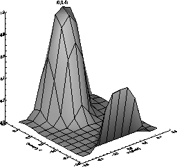
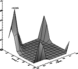
We can assemble all the 13-element vectors for each sub-pixel position into a 13-plane-deep 3-D array, each plane representing the fractional grade distribution of a given grade across the pixel. Examples of these planes are given in Figures 4.15 and 4.16. The peaks of the distributions are marked in the figures and given in Table 4.13 for each plane. We can treat these planes as probability distributions for each grade, showing the likelihood that a photon impinging at a certain sub-pixel position will yield an event of the shape (grade) being considered.

 

Figure 4.15: Single-pixel event position probability distribution on left; Two-pixel event position probability distribution on right.  

Note the bi-modality in these distributions - the upwards single-split distribution shown in Figure 4.15 (right side), for example. Some events that occurred near the lower edge of the pixel were detected as up splits - this is because enough of the charge clouds from these events were detected in the adjacent (lower) pixel that they were detected as upward splits. This illustrates the fact that we cannot know in which pixel the event really occurred, we can only assume that it occurred in the brightest pixel, and this assumption is not always right. Note also that, by replicating these single-pixel distributions for adjacent pixels, a consistent probability distribution appears, shaped similarly to the single-pixel distribution but centered on different sub-pixel coordinates ((0.3,-0.3) for the L-shaped events shown in Figure 4.16, instead of (0,0) for the single-pixel events) and having somewhat different widths. This implies that, if we are given an event's grade, we have a distribution showing the likelihood that the event came from a certain sub-pixel position.

 

Figure 4.16: Three-pixel (L-shaped) event position probability distribution on left; Four-pixel (square-shaped) event position probability distribution on right.  

Returning to the simulations, we deposited 4000 photons at the same sub-pixel position and came up with a distribution of grades. We want to use that distribution of grades to estimate the position of this ensemble of events. We have probability distributions of positions for each event, but how do we combine these to yield the best-estimate position for the ensemble?

As an initial step, we chose the simplest conceivable mapping. We assumed that a given grade came from a photon which interacted at the most likely sub-pixel position for that grade, i.e. wherever the peak is in the plots mentioned above. The sub-pixel coordinates of the peak are given as the third column of Table 4.13. Then we just averaged these positions to get the most likely sub-pixel position for the ensemble.

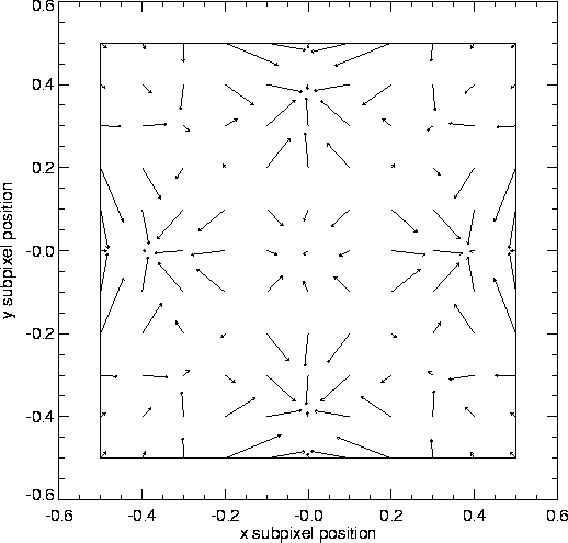
We computed ensemble position estimates as above for each sub-pixel position. Then to test the accuracy of the method, we generated a ``distortion map'' by subtracting the true position from the estimated position (separately for x and y), then computing a radial distortion. Figure 4.17 shows the distortion map for the lower left pixel quadrant. This map is intended to illustrate the degree to which this simple algorithm is able to recover positions. Note that there are regions on the pixel where the algorithm works well, and regions where it does not. This leads to ambiguities in a photon's true sub-pixel position and indicates that this algorithm provides accurate sub-pixel positioning to about 1/16 pixel.

 

Figure 4.17: Radial distortion map for one quadrant of a pixel, showing the difference between the true (base of arrow) and reconstructed (head of arrow) positions for 36 sample positions in a pixel.  

A more relevant test of the algorithm is the degree to which it can recover an accurate sub-pixel position of a point source smeared by a PSF. To simulate this, we generated photons with a two-dimensional Gaussian distribution about some pre-determined sub-pixel position. We deposited these photons on simulated CCD frames one at a time, then simulated frame readout and event detection and grading. This rate of one photon per source per frame is consistent with the readout rate expected for modest sources with AXAF. Using each event's grade as above, and ignoring events with grades S+, P+, and Other, we assigned to the event a sub-pixel position (the most likely position for that grade). Once we had accumulated an ensemble of events, we computed the simple average and standard deviation for the x and y positions separately and compared these estimates of the source's position and the PSF widths to the input values. We also made these estimates using only integer pixel positions for each photon and using the true sub-pixel positions for each photon, for comparison. Since the positions and PSF widths obtained from the true sub-pixel positions of the photons are the best estimates we can make given the finite sample size, the fairest comparison is between these results and those for the two algorithms in question, not between the input values and the results for the two algorithms. The results are summarized in Table 4.14. Note that some source positions were deliberately located at sub-pixel positions that suffered large distortions in the earlier tests (see Figure 4.17).

 

Energy # of 4c|True PSF 4c| Estimate Using 4c|Estimate Using 4c| Estimate Using

(eV) photons 4c| 4c|Integer Pixel Pos. 4c|Mapped Sub-pixel Pos. 4c|Real Photon Pos.

$$\sigma_{x} \sigma_{y} \sigma_{x} \sigma_{y} \sigma_{x} \sigma_{y} \sigma_{x} \sigma_{y}$$ x y x y x y x y

1000 3000 5.30 5.00 0.85 0.85 5.30 5.00 0.90 0.89 5.30 5.00 0.85 0.86 5.30 5.00 0.85 0.85

1000 3000 5.38 5.35 0.85 0.85 5.37 5.34 0.90 0.89 5.37 5.34 0.85 0.85 5.37 5.34 0.84 0.85

1000 3000 5.20 5.50 0.85 0.85 5.18 5.48 0.90 0.91 5.18 5.49 0.85 0.87 5.18 5.49 0.84 0.86

1000 500 5.20 5.50 0.85 0.85 5.21 5.51 0.89 0.90 5.20 5.52 0.84 0.87 5.20 5.52 0.83 0.86

1000 100 5.20 5.50 0.85 0.85 5.31 5.45 0.94 0.83 5.25 5.51 0.86 0.80 5.25 5.50 0.88 0.80

1000 1000 5.05 5.35 0.85 0.85 5.03 5.30 0.88 0.90 5.07 5.30 0.84 0.86 5.06 5.30 0.84 0.86

500 1000 5.05 5.35 0.85 0.85 4.96 5.31 1.02 1.03 4.97 5.30 1.00 1.01 5.02 5.37 0.85 0.85

5000 1000 5.05 5.35 0.85 0.85 5.08 5.33 0.91 0.89 5.10 5.34 0.88 0.86 5.09 5.34 0.86 0.85

1000 1000 5.03 5.35 0.10 0.10 5.18 5.50 0.47 0.00 5.05 5.38 0.13 0.16 5.05 5.38 0.10 0.10

5000 1000 5.03 5.35 0.10 0.10 5.18 5.50 0.47 0.00 5.04 5.30 0.12 0.18 5.05 5.35 0.10 0.10

1000 1000 5.05 5.35 0.40 0.40 5.07 5.36 0.51 0.49 5.07 5.35 0.40 0.42 5.07 5.35 0.40 0.41

1000 20 5.05 5.35 0.40 0.40 5.00 5.45 0.51 0.51 5.02 5.48 0.42 0.40 5.08 5.43 0.37 0.40

1000 5 5.05 5.35 0.40 0.40 5.30 5.50 0.45 0.71 5.30 5.42 0.35 0.48 5.27 5.35 0.30 0.47

These results confirm that the sub-pixel position mapping algorithm described above does a better job of recovering the source position than integer pixel positioning, when the PSF is small compared to the pixel size. Not surprisingly, the algorithms converge when the PSF is comparable to the pixel size (as we approach critical sampling). The results of the grade-based algorithm are affected by energy since the splitting is affected by energy - as fewer events are split, the sub-pixel position mapping algorithm collapses to integer pixel positioning. Sub-pixel position mapping appears to perform marginally better than integer pixel positioning for small numbers of photons.

  

Figure 4.18: Astrophysical spectrum predicted without radiation damage

  

Figure 4.19: Astrophysical spectrum predicted with 8 cm of Al shielding thickness

  

Figure 4.20: Astrophysical spectrum predicted with 4 cm of Al shielding thickness